Maximum Entropy Inverse Reinforcement Learning: Understanding the Trajectory Formula

Inverse reinforcement learning (IRL) asks a different question from classical RL: instead of assuming a reward function and learning a policy, you observe expert behavior and infer what reward would make that behavior look rational. One of the cleanest probabilistic formulations is the maximum entropy trajectory model. This post is a practical engineering note on what the formula means, why entropy matters, and where the Markov decision process (MDP) shows up under the hood.

Markov Diagram

The formula

Over candidate trajectories $T_i$, the model defines:

$$ P(T_i \mid \mathbf{w}) = \frac{1}{Z(\mathbf{w})} \exp\Bigl( \sum_{(s,a) \in T_i} \mathbf{w} \cdot \boldsymbol{\phi}(s,a) \Bigr) $$

$T_i$ — a complete trajectory (a sequence of state–action pairs).
$\mathbf{w}$ — a weight vector; in linear IRL, $\mathbf{w}$ parameterizes the implied reward $R(s,a) = \mathbf{w} \cdot \boldsymbol{\phi}(s,a)$.
$\boldsymbol{\phi}(s,a)$ — a feature vector for taking action $a$ in state $s$ (progress toward a goal, proximity to obstacles, smoothness, etc.).
$\mathbf{w} \cdot \boldsymbol{\phi}(s,a)$ — scalar reward contribution for one step.
$\sum_{(s,a) \in T_i} \mathbf{w} \cdot \boldsymbol{\phi}(s,a)$ — trajectory score (total reward along the path).
$Z(\mathbf{w})$ — the partition function: sum of $\exp(\text{score})$ over all trajectories so probabilities normalize to one.

Notation at a glance

Term	Meaning
$T_i$	One candidate trajectory, path, or behavior sequence
$\mathbf{w}$	Learned weights; defines the linear reward in this setup
$\boldsymbol{\phi}(s,a)$	Features for $(s,a)$: progress, risk, smoothness, compliance, …
$\mathbf{w} \cdot \boldsymbol{\phi}(s,a)$	Scalar reward for one step
$\sum_{(s,a) \in T_i}$	Sum of step rewards along the trajectory
$\exp(\cdot)$	Turns scores into positive, unnormalized masses
$Z(\mathbf{w})$	Normalizer over trajectories (the hard part in large spaces)

Intuition: a softmax over trajectories

Operationally, the recipe is:

Score each trajectory by summing $\mathbf{w} \cdot \boldsymbol{\phi}(s,a)$ along the path.
Exponentiate each score.
Divide by the sum of all exponentiated scores.

That is a softmax over trajectories: higher-scoring paths get higher probability, but nothing is forced to probability one unless the data and weights make that inevitable.

That matters for real experts. Demonstrations are rarely perfectly deterministic; several trajectories can be good. Maximum-entropy modeling keeps that uncertainty instead of collapsing everything onto a single “best” path.

IRL, MDPs, and feature matching

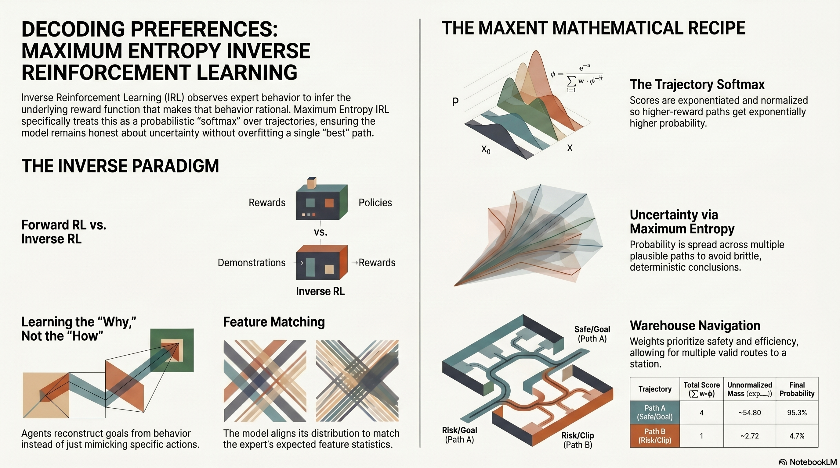
Forward RL: given dynamics and reward, find a good policy. IRL: given demonstrations, infer a reward (or reward parameters) that rationalizes them.

In maximum-entropy IRL, one assumes $R(s,a) = \mathbf{w} \cdot \boldsymbol{\phi}(s,a)$. The trajectory score is the sum of per-step rewards. Expert data are treated as if they were drawn from a distribution where higher-reward trajectories are exponentially more likely — exactly the Boltzmann form above.

Estimation goal: find $\mathbf{w}$ such that observed demonstrations are likely under $P(T \mid \mathbf{w})$. In practice, that means learning what the expert seems to care about — safety, efficiency, smooth motion, rule compliance — only through the features you encode.

A standard theoretical consequence is feature matching (in expectation): the model’s distribution aligns expected feature counts with those implied by the demonstrations. If experts consistently avoid obstacles and move smoothly, the inferred reward should induce similar statistics. Feature design is not cosmetic; it is the language in which preferences become identifiable.

Where the MDP enters

Trajectories $T_i$ are usually feasible paths in an environment: states, actions, and transitions. In the finite case, that is a finite MDP: discrete states and actions, and transitions $P(s' \mid s, a)$ constrain which sequences are valid. The formula does not print the transition table, but candidate trajectories are generated inside that structure. When the state space is huge, you cannot enumerate all trajectories; $Z(\mathbf{w})$ is approximated with dynamic programming, sampling, or other tractable surrogates — that is the central engineering bottleneck.

What “maximum entropy” means here

Entropy measures how spread out a distribution is. High entropy: mass over many trajectories. Low entropy: mass concentrated on a few.

Maximum entropy means: among all distributions that satisfy chosen constraints (typically, matching statistics of the demonstrations, especially feature expectations), pick the distribution that is otherwise least committal — it adds no extra assumptions beyond those constraints.

If several trajectories fit the data, probability should spread across them instead of assigning one path probability one and the rest zero. The exponential-family form is not arbitrary: it arises from maximizing entropy subject to feature-matching constraints. The same structure appears in maximum-entropy IRL, conditional random fields, Gibbs distributions, and softmax policies.

Tiny worked example (features and weights)

Suppose step-level features capture: progress toward goal, collision / obstacle contact, and smooth motion. A weight vector might be $\mathbf{w} = [2.0,\,-5.0,\,1.0]$: progress is good, collisions are strongly penalized, smoothness is mildly rewarded.

Trajectory A reaches the goal while avoiding obstacles → total score 6.
Trajectory B reaches the goal but clips an obstacle → total score 1.

Because $\exp(6) \gg \exp(1)$, A gets much higher probability under $P(T \mid \mathbf{w})$. B is not impossible — only less likely. That is the maximum-entropy mindset: bias toward what explains the expert, without zeroing out plausible alternatives.

Python: scores, partition function, probabilities

The snippet below scores a small finite set of candidate trajectories (enumeration is only toy-scale here).

import math

w = [0.8, -0.2]
T1 = [[1, 0], [0, 1], [1, 1]]
T2 = [[0, 1], [0, 1], [1, 0]]
T3 = [[1, 1], [1, 0]]
trajectories = [T1, T2, T3]


def dot(u, v):
    return sum(ui * vi for ui, vi in zip(u, v))


def trajectory_score(T, w):
    return sum(dot(w, phi) for phi in T)


scores = [trajectory_score(T, w) for T in trajectories]
unnorm = [math.exp(score) for score in scores]
Z = sum(unnorm)
probs = [u / Z for u in unnorm]

for i, (score, prob) in enumerate(zip(scores, probs), start=1):
    print(f"T{i}: score={score:.3f}, P(T{i}|w)={prob:.3f}")

Each step is a feature vector $\boldsymbol{\phi}$.
The trajectory score is $\sum \mathbf{w} \cdot \boldsymbol{\phi}$.
$\exp(\text{score})$ gives an unnormalized weight; $Z$ sums them; division yields valid probabilities.

A mobile robot moves to a packing station while avoiding shelves, slowing near people, and preferring smooth motion. A natural feature vector per $(s,a)$ might include: moves toward goal, close to obstacle, near human worker, smooth motion. Learned $\mathbf{w}$ encodes implicit priorities from demonstrations (positive weights reward preferred behavior, negative weights penalize risk or inefficiency).

Pipeline (conceptual):

Collect expert demonstrations (human teleop, planner traces, etc.).
Represent each trajectory by summing $\boldsymbol{\phi}(s,a)$ along the path (or equivalently summing $\mathbf{w}\cdot\boldsymbol{\phi}$ if optimizing $\mathbf{w}$).
Use $P(T \mid \mathbf{w}) \propto \exp(\sum \mathbf{w}\cdot\boldsymbol{\phi})$ so expert-like paths get higher mass.
Fit $\mathbf{w}$ so demonstrated trajectories are likely and expected features match the data.
Deploy the implied reward for planning in new layouts.

In a real warehouse, many paths can be safe. Maximum entropy avoids pretending there is a single “correct” route; it learns a reward that ranks paths while preserving uncertainty where data are ambiguous.

Feature (example)	Typical meaning
Moves toward goal	Progress to target
Close to obstacle	Penalize risk near shelves or walls
Near human worker	Tighter safety margin
Smooth motion	Predictable, executable motion

Numerical walkthrough (two trajectories, two features)

Let $\boldsymbol{\phi}(s,a) = [\text{towardGoal}, \text{energyCost}]$ and $\mathbf{w} = [2,\,-1]$: reward progress toward the goal, penalize energy.

Two toy three-step trajectories (chosen by hand for readability — in real IRL they would come from demos, simulation, or a planner):

Trajectory	Step 1 $\boldsymbol{\phi}$	Step 2 $\boldsymbol{\phi}$	Step 3 $\boldsymbol{\phi}$	Total score $\sum \mathbf{w}\cdot\boldsymbol{\phi}$
$T_1$	$[1,1]$	$[1,0]$	$[1,1]$	4
$T_2$	$[1,1]$	$[0,1]$	$[1,1]$	1

Step scores for $T_1$: $1,\,2,\,1$ → sum 4. For $T_2$: $1,\,-1,\,1$ → sum 1.

Unnormalized weights: $\exp(4) \approx 54.60$, $\exp(1) \approx 2.72$. So $Z(\mathbf{w}) \approx 57.32$, and

$$ P(T_1 \mid \mathbf{w}) \approx 0.953,\qquad P(T_2 \mid \mathbf{w}) \approx 0.047. $$

The lower-scoring trajectory is unlikely but not zero — by design.

import math

w = [2, -1]
T1 = [[1, 1], [1, 0], [1, 1]]
T2 = [[1, 1], [0, 1], [1, 1]]


def dot(a, b):
    return sum(x * y for x, y in zip(a, b))


def score(T, w):
    return sum(dot(w, phi) for phi in T)


s1, s2 = score(T1, w), score(T2, w)
e1, e2 = math.exp(s1), math.exp(s2)
Z = e1 + e2
print(round(e1 / Z, 3), round(e2 / Z, 3))  # 0.953, 0.047

Engineering takeaways

Takeaway	Why it matters
Feature quality dominates	Weak or wrong features → weak or misleading inferred rewards.
Maximum entropy reduces brittleness	Multiple near-optimal behaviors can coexist instead of a forced deterministic story.
$Z(\mathbf{w})$ is the hard part	Exact enumeration is intractable in large MDPs; implementations use DP, sampling, or approximations.
IRL targets objectives, not only actions	A learned reward often generalizes to new situations better than pure behavior cloning — when the model is right.

Where else this pattern appears

The same score then normalize structure shows up wherever you need a distribution over structured sequences: imitation learning under ambiguity, trajectory prediction in driving, user / gameplay sequence modeling, and structured prediction in ML (exponential models over outputs). The unifying pattern: meaningful features, learned weights, trajectory scores, and a normalized probability over candidates.

Bottom line

The maximum-entropy trajectory model gives a precise way to say: expert-like trajectories should be more probable when they score higher under a hidden linear reward, while the model stays honest about uncertainty when the data do not support a sharper conclusion.

For builders: define features carefully, infer $\mathbf{w}$ so demonstrations and feature statistics are explained, and use the maximum-entropy distribution to avoid overfitting a single story to limited data.

References

Ziebart, B. D., Maas, A. L., Bagnell, J. A., & Dey, A. K. “Maximum entropy inverse reinforcement learning.” AAAI, 2008.
Ng, A. Y., & Russell, S. “Algorithms for inverse reinforcement learning.” ICML, 2000.
Sutton, R. S., & Barto, A. G. Reinforcement Learning: An Introduction (2nd ed.). MIT Press, 2018. incompleteideas.net
Puterman, M. L. Markov Decision Processes: Discrete Stochastic Dynamic Programming. Wiley, 1994.

Trajectory	Step 1 \(\boldsymbol{\phi}\)	Step 2 \(\boldsymbol{\phi}\)	Step 3 \(\boldsymbol{\phi}\)	Total score \(\sum \mathbf{w}\cdot\boldsymbol{\phi}\)
\(T_1\)	\([1,1]\)	\([1,0]\)	\([1,1]\)	4
\(T_2\)	\([1,1]\)	\([0,1]\)	\([1,1]\)	1