The Wiener filter has a clean claim: among all linear filters operating on wide-sense stationary input, it produces the minimum mean-square estimation error. That claim has a closed-form proof, and the proof is short enough to walk through completely.
This post derives the Minimum Mean-Square Error (MMSE) starting from the cost function, through the Wiener-Hopf equation, to the final result. Every step is explicit. If you have worked with adaptive filters (LMS, NLMS, RLS), this is the deterministic optimum those algorithms approach iteratively without knowing the statistics in advance.
A companion lab implements the full derivation in MATLAB, Python, C, and C++: MMSE-Wiener-Filter-Lab.
Setup and notation
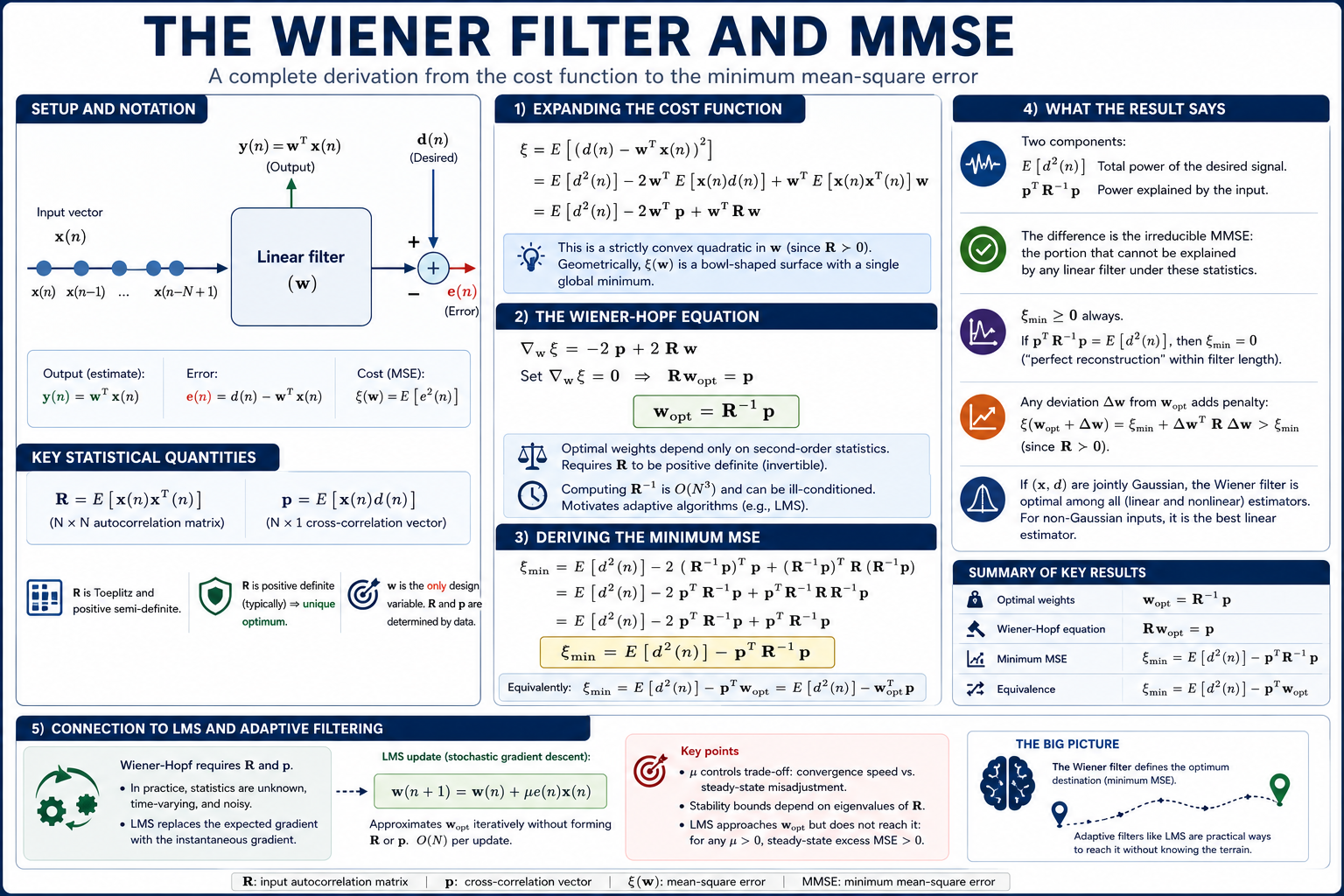
A linear filter with weight vector \(\mathbf{w}\) of length \(N\) receives input vector \(\mathbf{x}(n)\) and produces the estimate:
\[ y(n) = \mathbf{w}^T \mathbf{x}(n) \]The desired (target) signal is \(d(n)\). The estimation error is:
\[ e(n) = d(n) - y(n) = d(n) - \mathbf{w}^T \mathbf{x}(n) \]The filter’s job is to choose \(\mathbf{w}\) so that \(e(n)\) is as small as possible in a statistical sense. For real-valued signals, the cost function is the mean-square error:
\[ \xi(\mathbf{w}) = E\!\left[e^2(n)\right] \]Two statistical quantities determine everything that follows:
| Symbol | Definition | Structure |
|---|---|---|
| \(\mathbf{R}\) | \(E[\mathbf{x}(n)\mathbf{x}^T(n)]\) | \(N \times N\) autocorrelation matrix of the input |
| \(\mathbf{p}\) | \(E[\mathbf{x}(n)\,d(n)]\) | \(N \times 1\) cross-correlation between input and desired signal |
For a wide-sense stationary process, \(\mathbf{R}\) is Toeplitz and positive semi-definite by construction. It is positive definite when no sample in the observation window is a perfect linear combination of the others. That non-degeneracy condition is what guarantees a unique optimum.
Expanding the cost function
Start from the definition and expand the square:
\[ \xi = E\!\left[(d(n) - \mathbf{w}^T \mathbf{x}(n))^2\right] \]\[ = E\!\left[d^2(n)\right] - 2\,\mathbf{w}^T E\!\left[\mathbf{x}(n)\,d(n)\right] + \mathbf{w}^T E\!\left[\mathbf{x}(n)\mathbf{x}^T(n)\right]\mathbf{w} \]Substituting the definitions of \(\mathbf{p}\) and \(\mathbf{R}\):
\[ \xi = E\!\left[d^2(n)\right] - 2\,\mathbf{w}^T \mathbf{p} + \mathbf{w}^T \mathbf{R}\,\mathbf{w} \]This is a scalar-valued quadratic in \(\mathbf{w}\). The first term, \(E[d^2(n)]\), is the variance (power) of the desired signal, fixed by the data. The second and third terms depend on \(\mathbf{w}\). Because \(\mathbf{R}\) is positive definite, \(\xi(\mathbf{w})\) is strictly convex with a single global minimum. Geometrically, it is a bowl-shaped surface in \(N\)-dimensional weight space.
The weight vector \(\mathbf{w}\) is the only thing under the designer’s control. \(\mathbf{R}\) and \(\mathbf{p}\) are determined by the signal environment.
The Wiener-Hopf equation
The minimum of a differentiable convex function is where the gradient vanishes. Taking the gradient of \(\xi\) with respect to \(\mathbf{w}\):
\[ \nabla_{\mathbf{w}}\,\xi = -2\,\mathbf{p} + 2\,\mathbf{R}\,\mathbf{w} \]Setting to zero and solving for the optimal weight vector:
\[ \mathbf{R}\,\mathbf{w}_{\text{opt}} = \mathbf{p} \]\[ \mathbf{w}_{\text{opt}} = \mathbf{R}^{-1}\,\mathbf{p} \]This is the Wiener-Hopf equation [1][2]. It has a unique solution when \(\mathbf{R}\) is positive definite (and therefore invertible). The optimal weights depend only on the second-order statistics of the input and the cross-statistics between input and desired signal. No higher-order moments are needed.
One thing to note about practice: computing \(\mathbf{R}^{-1}\) directly is \(O(N^3)\) and numerically fragile when the eigenvalue spread of \(\mathbf{R}\) is large (ill-conditioned input). This is a primary motivation for adaptive algorithms. LMS approximates \(\mathbf{w}_{\text{opt}}\) iteratively at \(O(N)\) per update, without ever forming or inverting \(\mathbf{R}\).
Deriving the minimum MSE
To find the error floor, substitute \(\mathbf{w}_{\text{opt}} = \mathbf{R}^{-1}\mathbf{p}\) back into the cost function:
\[ \xi_{\min} = E\!\left[d^2(n)\right] - 2\,(\mathbf{R}^{-1}\mathbf{p})^T\,\mathbf{p} + (\mathbf{R}^{-1}\mathbf{p})^T\,\mathbf{R}\,(\mathbf{R}^{-1}\mathbf{p}) \]The simplification uses three properties of real-valued autocorrelation matrices. The transpose of a product reverses order: \((\mathbf{AB})^T = \mathbf{B}^T\mathbf{A}^T\). The matrix \(\mathbf{R}\) is symmetric (\(\mathbf{R} = \mathbf{R}^T\)), so its inverse is also symmetric: \((\mathbf{R}^{-1})^T = \mathbf{R}^{-1}\). And a matrix times its own inverse yields the identity: \(\mathbf{R}^{-1}\mathbf{R} = \mathbf{I}\).
Apply these to the second term:
\[ -2\,(\mathbf{R}^{-1}\mathbf{p})^T\mathbf{p} = -2\,\mathbf{p}^T(\mathbf{R}^{-1})^T\mathbf{p} = -2\,\mathbf{p}^T\mathbf{R}^{-1}\mathbf{p} \]And the third term:
\[ (\mathbf{R}^{-1}\mathbf{p})^T\,\mathbf{R}\,(\mathbf{R}^{-1}\mathbf{p}) = \mathbf{p}^T\mathbf{R}^{-1}\,\mathbf{R}\,\mathbf{R}^{-1}\mathbf{p} = \mathbf{p}^T\,(\mathbf{I})\,\mathbf{R}^{-1}\mathbf{p} = \mathbf{p}^T\,\mathbf{R}^{-1}\,\mathbf{p} \]The second term contributes \(-2\,\mathbf{p}^T\mathbf{R}^{-1}\mathbf{p}\). The third contributes \(+\mathbf{p}^T\mathbf{R}^{-1}\mathbf{p}\). They partially cancel:
\[ \boxed{\xi_{\min} = E\!\left[d^2(n)\right] - \mathbf{p}^T\,\mathbf{R}^{-1}\,\mathbf{p}} \]Since \(\mathbf{R}^{-1}\mathbf{p} = \mathbf{w}_{\text{opt}}\), this is equivalently:
\[ \xi_{\min} = E\!\left[d^2(n)\right] - \mathbf{p}^T\,\mathbf{w}_{\text{opt}} \]The quantity \(\mathbf{p}^T \mathbf{w}_{\text{opt}}\) is a scalar, so it equals its own transpose \(\mathbf{w}_{\text{opt}}^T \mathbf{p}\). Both forms appear in the literature [2][3].
What the result says
The MMSE has two components. The first, \(E[d^2(n)]\), is the total power of the signal you are trying to estimate. The second, \(\mathbf{p}^T \mathbf{R}^{-1} \mathbf{p}\), is the portion of that power the filter can explain using the input data. The difference is what remains unexplained: the irreducible estimation error for any linear filter under these statistics.
The MSE cannot go negative. If \(\mathbf{p}^T \mathbf{R}^{-1} \mathbf{p} = E[d^2(n)]\), the filter reconstructs the desired signal with zero error. That happens when \(d(n)\) lies entirely in the column span of the input observation matrix. In a channel equalization context, it means the channel distortion is fully invertible within the filter’s tap length.
\(\xi_{\min}\) is a hard bound on linear estimators. Deviating from \(\mathbf{w}_{\text{opt}}\) by any \(\Delta\mathbf{w}\) adds a penalty of \(\Delta\mathbf{w}^T \mathbf{R}\,\Delta\mathbf{w}\) to the error. Because \(\mathbf{R}\) is positive definite, that penalty is always positive. Any weight vector other than \(\mathbf{w}_{\text{opt}}\) produces strictly higher MSE.
One more property worth stating explicitly: the Wiener filter is optimal among linear filters under MSE without requiring the input to be Gaussian. If the input and desired signal happen to be jointly Gaussian, the conditional expectation \(E[d(n)|\mathbf{x}(n)]\) is itself linear, and the Wiener filter becomes optimal among all estimators, linear and nonlinear [2, Ch. 2][5]. For non-Gaussian inputs, nonlinear estimators can potentially do better, but the Wiener filter remains the best you can do with a linear structure.
Connection to LMS and adaptive filtering
The Wiener-Hopf equation requires \(\mathbf{R}\) and \(\mathbf{p}\) in closed form. In most real systems (equalizers, echo cancellers, noise reduction) you do not have these. The channel changes. The statistics drift. Estimating \(\mathbf{R}\) from finite data and inverting it is both noisy and expensive.
LMS sidesteps the problem by replacing the expected gradient \(-2\mathbf{p} + 2\mathbf{R}\mathbf{w}\) with the instantaneous gradient \(-2\,e(n)\,\mathbf{x}(n)\), then taking a small step at each sample:
\[ \mathbf{w}(n+1) = \mathbf{w}(n) + \mu\,e(n)\,\mathbf{x}(n) \]This is stochastic gradient descent on \(\xi\). The noise in the gradient estimate is the cost of not needing \(\mathbf{R}\) and \(\mathbf{p}\). The step size \(\mu\) controls the trade-off between convergence speed and steady-state misadjustment, and its stability bounds depend on the eigenvalue spread of the same \(\mathbf{R}\) that the Wiener-Hopf equation inverts directly [2, Ch. 5][3].
The Wiener filter defines the destination. LMS is one way to get there without knowing the terrain. The MMSE is the floor that LMS approaches but does not reach: for any \(\mu > 0\), the steady-state excess MSE is strictly positive. That gap is the price of real-time adaptation.
Lab
The full derivation is implemented in MATLAB, Python, C, and C++ in the companion repository: MMSE-Wiener-Filter-Lab.
References
- N. Wiener, Extrapolation, Interpolation, and Smoothing of Stationary Time Series, MIT Press, 1949.
- S. Haykin, Adaptive Filter Theory, 5th ed., Pearson, 2014.
- B. Widrow and S. D. Stearns, Adaptive Signal Processing, Prentice Hall, 1985.
- A. V. Oppenheim and R. W. Schafer, Discrete-Time Signal Processing, 3rd ed., Pearson, 2010.
- S. M. Kay, Fundamentals of Statistical Signal Processing, Vol. I: Estimation Theory, Prentice Hall, 1993.