Every communication system starts with the same goal: move a signal from one place to another and recover its meaning at the far end. In practice the signal passes through copper, air, fiber, antennas, amplifiers, filters, and ADCs. At each stage it picks up thermal noise, interference, quantization error, phase noise, and distortion.
By the time the waveform reaches the receiver, the question is not whether something arrived. The question is whether the useful signal is strong enough relative to the noise for the receiver to decide what was sent. That ratio is signal-to-noise ratio (SNR).
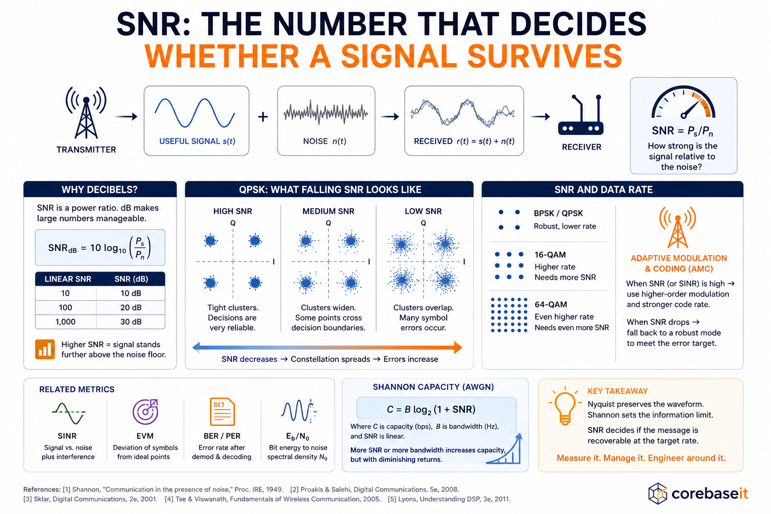
The diagram above ties the pieces together: SNR as a power ratio, what falling SNR does to a QPSK constellation, why higher-order QAM needs more margin, and where Shannon capacity sets the ceiling.
What SNR measures
SNR compares signal power to noise power:
$$ \mathrm{SNR} = \frac{P_s}{P_n} $$When \(P_s \gg P_n\), symbol decisions are reliable. When the two powers are comparable, the receiver is guessing. When noise dominates, the message is buried.
SNR is therefore both a measurement and a statement about decision confidence. Communication receivers are, at bottom, machines that infer which symbol or bit was transmitted from a noisy observation.
Why engineers use decibels
Power ratios in radio links span enormous dynamic range. Expressing SNR in decibels keeps the arithmetic manageable:
$$ \mathrm{SNR}_{\mathrm{dB}} = 10 \log_{10}\left(\frac{P_s}{P_n}\right) $$Each 10 dB step is a tenfold change in power ratio:
| Linear SNR | SNR (dB) |
|---|---|
| 10 | 10 |
| 100 | 20 |
| 1,000 | 30 |
Link budgets, antenna gains, cable losses, and amplifier noise figures are almost always handled in dB for this reason. The underlying idea stays simple: higher SNR means the signal stands farther above the noise floor.
The received signal and the QPSK picture
A simplified continuous-time model of what the receiver sees is:
$$ r(t) = s(t) + n(t) $$The receiver must map each observation \(r(t)\) (or its sampled form) to the most likely transmitted symbol. Small noise keeps the sample near the correct decision region. Large noise pushes it toward a neighbor. That is where bit errors start.
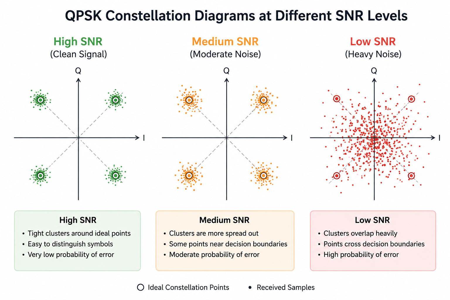
QPSK maps two bits to one of four phases in the I/Q plane. At high SNR, received points cluster tightly around the ideal corners. As SNR falls, the clouds spread. Points cross the I/Q axes that separate symbols, and the demodulator starts flipping bits. The symbol energy is still present; the evidence for which symbol it was is not.
Confirmed: Constellation spreading with falling SNR is the standard AWGN intuition for square QAM and PSK families.
Nuance: Real channels add fading, frequency offset, and ISI. Constellation diagrams then show rotation, elliptical spreading, or smeared trajectories — not just larger circular clouds. SNR alone does not fully describe those impairments.
SNR and data rate
SNR also limits how aggressively a link can modulate.
BPSK and QPSK place constellation points far apart relative to bits per symbol. They tolerate lower SNR. Higher-order formats — 16-QAM, 64-QAM, 256-QAM — pack more bits into the same bandwidth by moving points closer together. Spectral efficiency rises. Noise margin falls.
That trade-off shows up in adaptive modulation and coding (AMC) in Wi-Fi, LTE, and 5G: when measured SNR (or SINR) is high, the link selects a higher-order modulation and a stronger code rate; when it drops, the stack retreats to a robust mode. That fallback is not waste. It is the system staying inside a BER or BLER target.
Connection to Shannon capacity
SNR enters Shannon’s capacity formula for an AWGN channel with bandwidth \(B\):
$$ C = B \log_2(1 + \mathrm{SNR}) $$Here \(\mathrm{SNR}\) is a linear power ratio, not a dB value. Bandwidth and SNR both lift capacity, but the log term means returns diminish: doubling transmit power does not double capacity. At high SNR, capacity grows roughly as \(\log_2(\mathrm{SNR})\).
Confirmed: Shannon’s bound sets a theoretical ceiling for reliable rate on a noisy channel [1][2].
Interpretation: Pushing more bits per second through a fixed band requires more SNR, more bandwidth, stronger coding gain, or some combination. There is no free margin once you are near the bound.
In deployed systems, raising transmit power is only one lever — and often not the best. Regulatory EIRP limits, battery drain, PA nonlinearity, and co-channel interference all cap how far “turn it up” can go. Filtering, FEC, MIMO, equalization, and better channel estimation usually share the workload with power.
Not every “SNR” is the same number
SNR is quoted at many points in a receiver chain:
- At the antenna port
- After the LNA
- After channel filtering
- At the ADC
- After digital gain and correction
Related metrics answer slightly different questions:
| Metric | What it emphasizes |
|---|---|
| \(\mathrm{SINR}\) | Signal vs. noise plus interference |
| \(\mathrm{EVM}\) | How far received symbols deviate from ideal constellation points |
| \(\mathrm{BER}\) / \(\mathrm{PER}\) | End-to-end error rate after demodulation and decoding |
| \(E_b/N_0\) | Bit energy relative to noise spectral density \(N_0\) |
\(E_b/N_0\) is the usual figure for comparing modulation and coding schemes on an AWGN reference channel. It ties to SNR through data rate and bandwidth; they are not interchangeable without stating assumptions.
A headline SNR can look acceptable while the link still fails — for example, when phase noise rotates the constellation, timing error shifts samples, co-channel interference raises the effective noise floor, or channel-estimation error smears the reference. EVM, BER, and SINR often localize the failure better than a single RF SNR number.
What falling SNR looks like in practice
On a QPSK link, high SNR gives four separated clusters and negligible errors. Medium SNR widens the clusters; most symbols still decode, but edge cases near boundaries fail. Low SNR produces overlapping clouds: the demodulator runs, yet BER climbs, packets retry, and throughput collapses. To the user it feels like a slow connection. To the receiver it is a maximum-likelihood decision with weak evidence.
The same pattern appears across domains — Wi-Fi rate adaptation, cellular handover margins, satellite link closures in rain fade, optical OSNR limits, and ADC dynamic range before quantization noise dominates.
References
C. E. Shannon, “Communication in the presence of noise,” Proceedings of the IRE, vol. 37, no. 1, pp. 10–21, Jan. 1949.
J. G. Proakis and M. Salehi, Digital Communications, 5th ed. McGraw-Hill, 2008. (SNR, modulation, and AWGN channel performance.)
B. Sklar, Digital Communications: Fundamentals and Applications, 2nd ed. Prentice Hall, 2001. (Constellation diagrams, \(E_b/N_0\), and link budgets.)
D. Tse and P. Viswanath, Fundamentals of Wireless Communication. Cambridge University Press, 2005. (SINR, fading, and adaptive modulation.)
R. G. Lyons, Understanding Digital Signal Processing, 3rd ed. Pearson, 2011. (SNR in sampled and quantized systems.)
Further reading
- Nyquist is not Shannon: why more samples does not mean more information — sampling vs. channel capacity
- Why your internet has a speed limit — thermal noise and the physical noise floor
- Deriving MMSE: what the Wiener filter actually minimizes — optimal linear estimation under noise